

How To Draw Economic Graphs In Word
Easily-on Tutorials
Using pgfplots to make economical graphs in LaTeX
An approachable guide to making sleek, professional graphs in the industry standard typesetting language
one. Introduction
Economic science makes an arable employ of graphs to illustrate important concepts and phenomena. Yet the first matter ane may notice when typing up a paper in the field is the difficulty of making these graphs using word processors. That is where LaTeX comes in. This guide volition explain how we can use the pgfplots package to make elegant economical graphs in LaTeX.
one.ane. New to LaTeX?
Some readers may be unfamiliar with LaTeX. It is a powerful typesetting language capable of typesetting text, mathematical formulas, tables, and many other elements that word processors such as Word and Google Docs are incapable of. Its capabilities are extended by packages. This guide volition focus on making graphs with a bundle designed for plotting graphs — pgfplots — which itself relies on a parcel designed for making graphics — TikZ.
Along with LaTeX'due south formidable ability and customizability comes with it a reputable learning curve. Practice not despair. This guide was written under the assumption that readers are familiar with the very basics of LaTeX — but no more than that. (In Section 8: Resource, there are resource you lot can use to prepare and learn the basics of LaTeX.) If you tin can create a text document, load in packages, and write an equation in LaTeX's display math way, you demand not know annihilation else. Although if yous are already familiar with pgfplots and TikZ, yous may notwithstanding find some of the techniques used here useful for the very specific features of economic graphs.
i.ii. GitHub project repository
All of the finished graphs shown here are available on the GitHub repository for this guide. You can access the repository at https://github.com/jackypacky/pgf-econ-graphs. There, the TeX source codes and PDFs of all the graphs tin be found.
i.3. Packages
Nosotros will be using pgfplots to draw economic graphs, and so the pgfplots package should exist called. This will call TikZ and xcolor every bit well. Since we want to be able to shade in areas under curves, the fillbetween pgfplots library should exist called. Since we want to be able to specify positions effectually coordinates and employ a diversity arrowheads in TikZ, the positioning and arrows.meta TikZ libraries should be called equally well. Also, since we want to be able to utilize LaTeX's math style, we demand to call the amsmath package. In total, we have the following code snippet at the beginning of the certificate:
Out of personal preference, we will be using the Times New Roman 12 point font with a ane.25 line spread (which corresponds to a i-and-a-one-half line spacing). Then we will be using this certificate preamble:
2. Outlining the axes
To begin, nosotros demand to describe the axes on which our economic graphs will be drawn. Since pgfplots is a dependency of TikZ, we need to open and close the TikZ environment with \begin{tikzpicture} and \end{tikzpicture}. Within this surround, to construct the pgfplots environs, we insert \begin{axis} and \end{axis}. Since, presumably, we want the economic graph to be in the center of the page, all of this should be in the center environs, with \begin{center} and \stop{center} encompassing the code. So we have:
For the axis environment, parameters impact the whole graph (i.e. scaling, centrality ticks, grid lines) while commands impose specific plots (i.east. functions, lines, coordinate points). 1 matter to note, syntactically, is that parameters are separated past commas — "," — while commands are separated by semicolons — ";".
2.1. The centrality environment
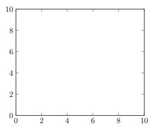
Before we tin can begin plotting functions, we need to specify which region of the Cartesian plane we wish to display. To specify the domain, we use the parameters xmin = 0 and xmax = x, where 0 and 10 are the minimum and maximum premises of the domain. Similarly, to specify the range, we use the parameters ymin = 0 and ymax = 10 to specify the minimum and maximum range bounds respectively. Then far, we have this code for the basic outline of the graph:
Running this code produces Figure 2–1.
2.2. Axis line directions
Nosotros need to make a couple modifications to brand this suitable for economic graphs. The default style of the graph frame is boxed, where blackness lines surround the graph on all sides. While this is good for line graphs and scatter plots — what pgfplots was built in mind for — economic graphs generally take an L-shaped frame. To modify the frame mode, we need to use the parameter axis lines = fashion, where the manner tin either exist left, correct, centre, box, or none. Figure two–2 shows some of these styles for the centrality lines.
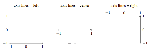
Clearly, nosotros need to employ axis lines = left as a parameter to make the L-shaped frame nearly economical graphs have. In add-on, the arrows at the end of the axes tin be removed by appending an asterisk to the end of the centrality lines so we apply, centrality lines* = left.
ii.3. Centrality ticks, scale, and clipping
Economic graphs typically practice not have numbers running forth the axes. This is considering most of them are theoretical diagrams and apply irrespective of the orders of magnitude involved. To this end, we need to remove the lines and numbers running along the 10 and y-axes — which are called axis ticks and axis tick labels respectively. The parameters that do this are xtick = {tick numbers} and ytick = {tick numbers} for the x and y-axes respectively. Within the curly braces after the xtick and ytick parameters, we put a listing of numbers separated past a comma which we want to run forth the respective axes. Since economic graphs, for the most role, keep the cipher at the bottom-left, nosotros will keep it in the x-ticks every bit such xtick = {0}. Since nosotros want no centrality ticks on the y-centrality, we write ytick = \empty. The case of an empty centrality ticks numbers list is a special case. Because pgfplots would utilize the default axis ticks if we had nothing within the curly braces, we need to specify that information technology is empty with \empty. To make non-blank centrality lines — for instance, graphs with specific, empirical values — Section four: Empirical curves covers filigree lines and axis ticks.
Considering the size of the effigy on the page, the default size is slightly too modest to present much illustration without cluttering the space available. To slightly increase the size of the graph, we write the parameter \scale = i.2. Of course, if you lot have a more complex or important illustration, a greater cistron can be used to create bigger graphs. On the other side, a lesser factor can be used to create smaller graphs. A scale cistron of 1.two occupies near a third of the page.
The terminal parameter we need to add is clip = fake. Normally, pgfplots cuts off any plots outside the graph, which is useful for automatically bounding functions. Nonetheless, we desire to be able to put labels outside the graph, and then nosotros disable that feature with this parameter. Instead, we volition be manually indicating the domain and range of plotted functions.
ii.4 Axis labels
Finally, the concluding consideration nosotros accept to accost earlier plotting anything on the graph are the centrality labels. Information technology is more than convenient to put them at the ends of axes instead of conventionally at the bottom (for the x-centrality) and to the left (for the y-axis) because nosotros want to use that space for other things (such equally variable labels and dimension lines). To put labels at the finish of the x and y-axes, the commands take the form of:
As a reminder, semicolons should exist at the end of these lines because they are commands every bit opposed to the parameters that have been used thus far. (Subsection 3.5: Labelling explains why this command works in more than item.) For the sit-in, we will utilize the 10 and y-axis labels of $x$ and $y$ respectively. Putting the dollar signs around the x and y puts them in LaTeX'south math way, allowing usa to write the mathematical expressions LaTeX is known for.
After all of these considerations are addressed, we cease upward with Figure 2–3:
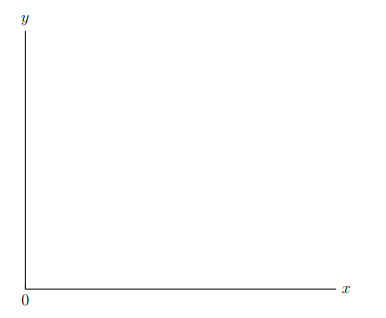
Now the graph is ready to have plots (e.one thousand. functions) drawn upon it. The code that produces Figure ii–3 is as follows:
three. Plotting, colours, and labelling (ex. indifference map and upkeep constraint)
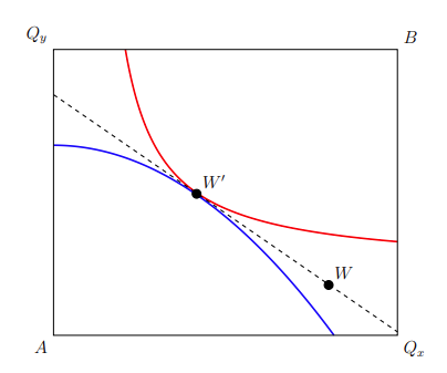
With our axes, we can begin drawing on the graph. Suppose we wanted to illustrate why demand is downward-sloping — meaning that quantity demanded falls as price rises — using indifference curves. More specifically, we want to plot an indifference map between good A and B with budget constraints showing an increase in the price of good A respective to a subtract in the quantity demanded of the proficient.
three.1 Plotting functions
First, we want to draw an indifference bend, U₁, defined past, say,
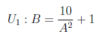
This is done past the post-obit control:
This is a long command. Let us have this in pieces. The addplot parameter of domain = min:max restricts the function graphed to the domain divisional by the minimum x-value, min (which is 0 in this case), and maximum x-value, max (which is 10 in this instance). Similarly, restrict y to domain = min:max restricts the function to the range bounded between min and max (which are 0 and x in this case). (Restricting y to a "domain" is a slight misnomer considering the proper mathematical term for the set of y-values is "range.") Annotation, the reason why we need to define the domain and range, as mentioned before, is that we disabled pgfplots'south clipping feature. The addplot parameter samples = n tells pgfplots to have a sure number of ten-values, n, at which to evaluate the function and draw a line through all the calculated coordinates. In do, the higher the number of samples, the smoother the plotted bend. The last addplot parameter, color = colour name, is cocky-explanatory. It colours the line to be the colour name. Colours are addressed in more than detail in the next subsection. In Subsection 3.ii: Colours, in that location is a list of the predefined colour names along with an caption on how to add more than predefined colour sets and ascertain new colour names.
Moving on to the mathematical expression within the curly braces, this is where we put the function's expression, 10/(x^two)+1. It is important to note that the conventional note of juxtaposition (placing numbers and letters side past side) for multiplication throws an error. Instead, an asterisk — "*" — can simply betoken multiplication. Otherwise, conventional reckoner notation applies, with improver, subtraction, division, and grouping represented by "+", "-", "/", and "( )" respectively. Plotting the aforementioned command yields Figure 3–one.
The code that produces Figure iii–1 is:
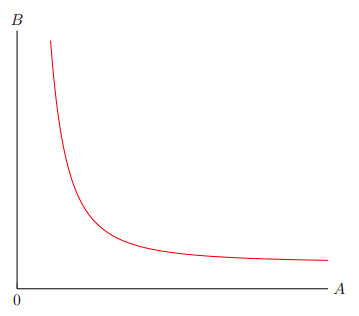
One thing to notice about Figure three–1 and its lawmaking is that the x-axis label is A and the y-centrality label is B. This is considering, in this instance, nosotros desire to prove that an increase in the price of good A causes a decrease in the quantity demanded of the good.
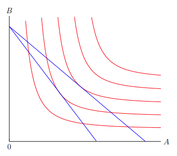
Naturally, an indifference map contains more than one curve. So, let united states of america plot multiple curves by translating the first curve to the right by one unit of measurement and up past i unit of measurement. In transformation notation, this corresponds to (x, y)→(10−1, y+1).
Successively using this transformation on U₁ produces U₂, U₃, U₄, and U₅,
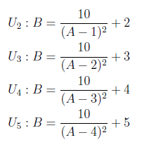
Plotting all v of these curves yields Figure 3–2.
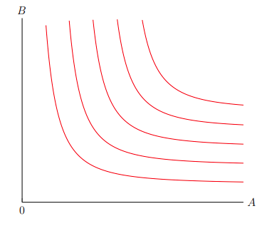
The indifference curves in Figure 3–2 are plotted by the following code snippet:
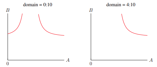
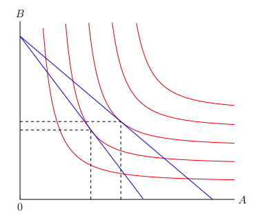
Notation that the domain restrictions are different for each function. U₁ is restricted to A ∈ (0, 10), while U₂ is restricted to A ∈ (1, x), and U₃ is restricted to A ∈ (2, ten), and then on. The reason for this is because each indifference curve's equation has different vertical asymptotes, with it being A = 0 for U₁, A = 1 for U₂, and A = two for U₃, etc. Considering we but intendance near the graph of the equation at the correct-hand side of the vertical asymptote, we restrict the utility functions to the domain right of the vertical asymptote. Figure 3–3 illustrates this domain restriction.
At present that we have the indifference map plotted, we need to plot the changing budget constraints in response to a ascent in the cost of adept A. In result, this means ii diagonal lines: one from a positive B-intercept to a positive A-intercept, and another line from that B-intercept to a reduced positive A-intercept. This represents the modify in the maximum number of skillful A that can be bought considering of a price increase, while the maximum number of good B remains the aforementioned. In addition, because nosotros want to show the modify in the consumer decisions after a constriction in budget constraint, the two budget constraints must be tangent to indifference curves. We will use U₃ to be tangent to the original budget constraint at A = 4.7 and U₂ to be tangent to the new one at A = 3.3. The original and new upkeep constraints are calculated to be the equations B = 9.16 − 1.02A and B = nine.xvi − i.59A respectively (these are approximations of the actual tangents). Logistically, the equations of these budget constraints can be calculated or approximated beforehand, manually or with software such as WolframAlpha or Desmos. (For instance, with WolframAlpha, the original budget constraint equation can found by inputting tangent at x = four.7 for y = 10/((x-two)^two)+3, which outputs y = nine.14744–1.01611x.) Using the same addplot control which we used previously to plot the lines of the indifference curves, we can plot the 2 budget constraints.
Lastly, to make the budget constraint lines stand up out in the midst of the indifference map, nosotros need to thicken them. This is washed by adding the parameter thick to the addplot. The preset line thicknesses are ultra thin, very thin, thin, thick, very thick, or ultra thick — or we could define our own thickness with the line width = width parameter where width is in units of length. In full, we accept the post-obit code snippet for the budget constraint lines:
Plotting them on the graph yields Figure 3–4.
iii.ii. Colours
In the previous subsection, we used two colours — carmine and bluish — to draw functions. Yous might be wondering how many colours we can use, or how to define new colours. Call up, nosotros called the xcolor package because it expands LaTeX'due south express base capacities to manipulate and use colours.
There are 19 default colours predefined past LaTeX:
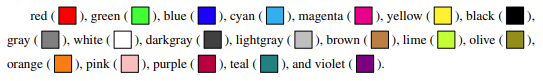
(I explain how to make these coloured squares in Subsection 6.ii, the command that produces a red square is \fcolorbox{black}{red}{\textcolor{red}{\rule{\fontcharht\font`X}{\fontcharht\font`Ten}}}.)
Nonetheless, if these colours are too limited, xcolor comes with a variety of options that defines more colours. For example, the dvipsnames option defines 68 more colours:
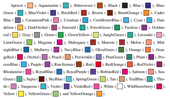
It is of import to note that these colour names are example-sensitive. Significant that color = violet is different from color = Violet, and color = VIOLET volition throw an error.
To add together the dvipsnames colour palette, we call the xcolor packet with the dvipsnames option, so, \usepackage[dvipsnames]{xcolor}. If the usepackage command is called afterward pgfplots's, an mistake volition exist thrown. This is considering TikZ calls xcolor by default and clashes with this new usepackage command. Then brand certain that the xcolor package is chosen earlier the TikZ packet. Alternatively, if this does not piece of work, then nosotros could add the parameter xcolor = {dvipsnames} to the certificate class command. For united states, nosotros would use, \documentclass[12pt, xcolor = {dvipsnames}]{article}.
There are other palettes aside from dvipsnames, such as svgnames, which defines 151 colours, or x11names which defines 317 colours. In add-on, new colours can be manually divers using the control \definecolor{name}{model}{variable i, variable 2, variable 3}, where the model is either rgb, HTML, cmyk, among others. For example, a lite tan colour tin exist defined by \definecolor {name}{rgb}{0.95, 0.95, 0.92}.
A lot can be done with colours in LaTeX. We can colour text, have groundwork colours, and make the page color different from the standard white (though that would exist ill advised, considering the strain on printers). Most of these are outside the telescopic of this guide and so volition not be covered. Resource are available at Section viii: Resource, which includes documentation and guides on the xcolor packet.
three.3. Plotting dashed line segments
Returning to the indifference map and upkeep constraints graph we were working on, the next step is to draw dashed lines on it. Pgfplots has a command for line graphs, wherein it will connect all inputted coordinates sequentially with a line going through them. The coordinates of the original decision indicate — where the original budget constraint is tangent to an indifference curve — are calculated to be (4.vii, 4.37). So the dashed line will go from (4.7, 0), the A-intercept, to (4.vii, 4.37), the decision point, to (0, iv.37), the B-intercept. The command that does this is as follows:
As seen, the coordinates the line goes through should be listed inside the curly braces. Also, considering we want the line to be dashed, nosotros include the parameter dashed. The other ii parameters, colour = black and thick accept already been covered in the previous subsections. They respectively colour the resulting line black and make its line width thicker. Repeating this procedure for the new decision indicate at (3.3, three.9) yields Figure 3–5.
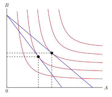
three.iv. Plotting coordinate points
Conveniently, imposing black coordinate points on the graph is very like to drawing a line. In fact, to make a besprinkle plot, pgfplots uses the same command that was previously used to draw connected line segments. Then two parameters are added. The beginning is marking = *, which draws a filled circle at every coordinate the line connects. Marks other than "*" can be used, such equally "x" , "+", "|", "o", (all of which look similar the character representing information technology), and many more marks. Second, to remove the line, we write the parameter just marks. In improver, to increase the size of the marks, we add the parameter mark size = 3. In total, nosotros take the following control to plot the coordinate points:
Using this command on the graph yields Figure 3–vi.
3.v. Labelling
Finally, to finish the graph we need to characterization all the relevant parts of information technology. Specifically, nosotros need to put letters near the A and B-intercepts, the coordinate points, and the ends of the functions. To label a role of the graph, the command takes the class of:
This command volition place some text, the label, side by side to the coordinate specified. In addition, where the label ends up near the coordinate depends on the position, it tin either be left, right, above, or below the coordinate. For instance, to put a characterization of Qₐ below (iv.7, 0), where the dashed line extending downward from the original determination point meets the A-axis, we write the following command:
We have already used a grade of the node command previously when labelling our axes. Discover, withal, that the coordinate point for an axis label is different considering it refers to the end of an axis. Using the labelling command to label the remainder of the graph, such equally the functions and coordinates, we terminate up with Figure 3–7.
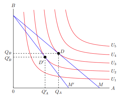
Finally, nosotros accept completed the indifference map illustrating why demand slopes downwards. It is considering Q′ₐ is less than Qₐ when the budget shifts from M to 1000′. More importantly, nosotros illustrated this in LaTeX! Figure iii–seven is produced past the following code, combining all of the elements covered in this department:
four. Empirical curves (ex. market equilibrium)
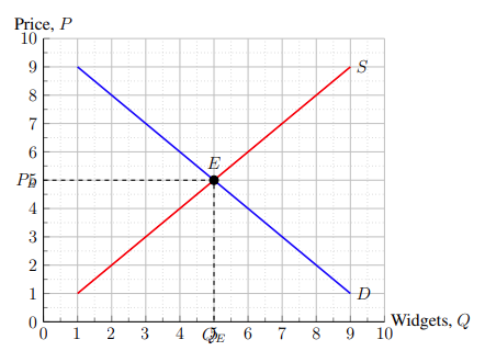
At the start of this guide, I assumed that we were working on a blank graph. Meaning, the x and y-centrality did not take whatsoever ticks because they do not have whatever values associated with them. These types of graphs are useful for theoretical models — applicative to relevant situations no matter the order of magnitude. Sometimes, nonetheless, we actually take empirical data. In this example, we might want grid lines on which to impose plots such as functions, coordinates, dashed lines, and so on. A couple modifications are needed to convert our "bare" graph to service empirical values. Specifically, we want to impose grid lines so work out the legibility problems such as distancing centrality labels and putting a white groundwork colour behind labels in the graph to avoid ataxia. Permit us transform a marketplace equilibrium curve, Figure 4–one, so that is able to reverberate empirical data.
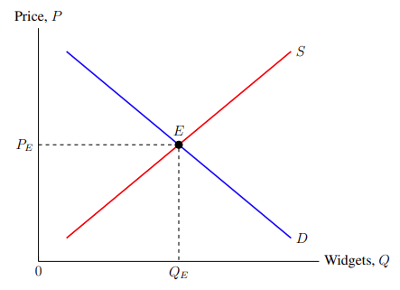
The elements in Effigy 4–1 accept been explained in previous sections. It is produced past the post-obit code:
four.ane. Major and minor grid lines
To start with, we want centrality ticks and numbers to run forth both axes. This was covered briefly in Subsection 2.3: Centrality ticks, scale, and clipping, but there we were focused on removing them. Equally a reminder, the axis parameters which control the ticks are xtick = {tick numbers} and ytick = {tick numbers}. Instead of them containing but 0 or existence empty, we desire them to exist the numbers which fit our information. In this instance, the set of tick numbers will be {0,ane,2,3,four,five,6, 7,8,nine,10} for both of them. Adjacent, nosotros want to impose grid lines upon the graph. We are still working with axis parameters, not commands. Usefully, in that location are two types of grid lines, major grid lines and minor grid lines. Major grid lines extend from the axis ticks and numbers. Meanwhile small grid lines extend from smaller ticks between major ticks and practice not have a number associated with them. They both have different styles and then tin aesthetically convey more than precision. To show both grids, include the axis parameter filigree = both. Similarly, if we desire only i or none of the grids, nosotros would use the value of major, minor, or none–though by default neither grid is shown. To set the number of minor ticks betwixt major ticks, the axis parameter pocket-size tick num = number is used, where the number is the number of pocket-sized ticks. In this case, we want one minor tick halfway between the major ticks — otherwise it would be too cluttered — so the number of minor ticks is 1. Moreover, nosotros want the major grid lines to be solid lines and the pocket-sized grid lines to exist dotted lines. This way, half and full increments are visually axiomatic. To modify the style of major and minor filigree lines to solid and dotted lines, we use grid style = solid and minor grid manner = dotted respectively. More styles include dashed, thin, and thick. Defining the grid style to exist solid is redundant since that is the default, merely I take opted to brand it explicit. So far we have added, or modified, the parameters in the following code snippet:
This snippet adds centrality ticks from 1 to x in increments of 1 on both the ten and y axes. In addition, it shows both the minor and major filigree lines, sets the number of small-scale ticks between major ticks to one tick, and makes major filigree lines solid lines and minor filigree lines dotted lines. Using these parameters to the blank market equilibrium graph results in Effigy 4–2.
Ah! That is ugly! While we got the centrality ticks and grid lines we were seeking, this acquired other problems for the legibility of this graph. Specifically, the labels of Qₑ and Pₑ demand to exist moved away from the axis numbers, the centrality labels should be moved slightly away from the graph, and the labels of E, Due south, and D demand to have white backgrounds to reduce ataxia. In add-on, in that location are two zeros at the origin — one is enough.
iv.ii. Distancing labels, colouring label backgrounds
Starting with the former effect, the ten and y-intercept labels demand to exist moved abroad from the graph to make room for the axis numbers. Think that labels take the form of:
While the position does a skillful job in most situations of determining how far the label should be from the coordinate, sometimes we want to increase this distance. In such situations, the distance can be specified with position = distance. And then, for example, the position for Qₑ can be changed to below = 10pt. Repeating this for the Pₑ label, we have the following code snippet:
Moving on to the latter problems. Getting rid of the y-axis label of 0 and moving the axis labels can both be done by irresolute the domain and range of the graph shown. To go rid of the 0 on the y-axis, we define the minimum of the range to exist 0.01 (any very minor number suffices, though this varies depending on the order of magnitude of the data). So we take ymin = 0.01 as an axis parameter. To distance the axis labels, the maximums of both the domain and range should exist extended to 10.5 (this besides varies depending on the order of magnitude). In sum, we have the following lawmaking snippet:
Finally, nosotros want to colour the background of labels on the graph white. Otherwise, we would be stuck with lines cutting through East, S, and D, which does not expect proficient. This also involves a relatively simple adjustment. Nosotros add the parameter fill = white to the node commands of the labels. The code snippet for the inverse labels are:
The label of E has likewise been distanced by v pt using the positioning parameter as explained in the preceding paragraph. This was washed to avert covering the supply and demand lines with the white groundwork. There are other ways to resolve this inconvenience. For example, considering pgfplots layers these plots sequentially — where later commands cover previous ones — simply having the node command for the label higher up the ones for the supply and demand line curves could work. That way, the commands for the supply and demand curves would exist executed after the label and would cover up the white background.
Combining all of these adjustments, we end up with Effigy 4–3.
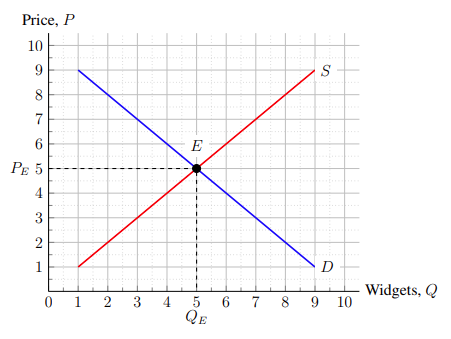
Then we have finished adjusting the blank graph to one with ticks and grid lines so that it can arrange empirical data and represent specific values. The lawmaking for Figure 4–iii is:
five. Shading, arrows, and graphs adjacent (ex. supply increase, price-taking business firm)
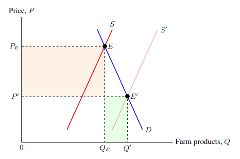
A lot tin can be washed by plotting curves, lines, and coordinate points. But sometimes we need to indicate out features or bespeak areas on the graph. This can be washed by drawing arrows and shading in areas on the graph with colour. Permit us apply these tools to illustrate the bumper harvest paradox: why farmers' incomes fall afterwards a bountiful harvest. A bumper harvest corresponds to a supply shift rightward in the market equilibrium graph where demand is relatively price-inelastic. This is depicted in Figure 5–ane.
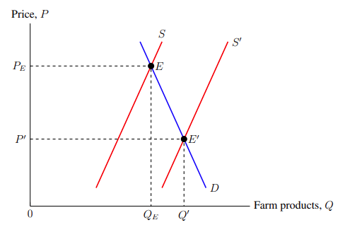
Effigy five–1 is graphed using the tools already explained in the sections to a higher place. The code is equally follows:
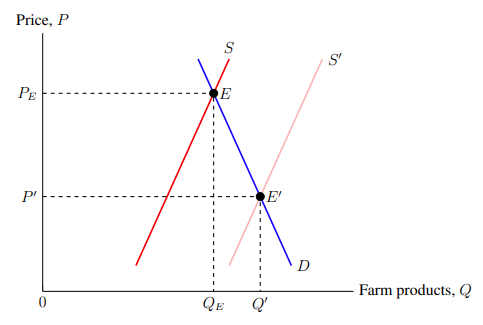
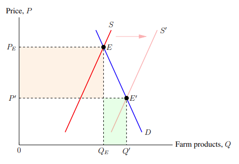
5.1. Opacity and transparency
Correct at present, both supply curves are the same opaque red. To make it evident which is the original supply bend and which is the new one, we will make the new one slightly transparent. Nosotros do this by adding the parameter opacity = opacity value to the addplot command, where the opacity value is the percent the plot is opaque ranging from 0, perfectly transparent, to 1, perfectly opaque. Making the new bend mostly transparent seems to brand it evident that it is new. So we write opacity = 0.3 for its addplot command. The outcome of making the new supply curve more transparent is shown in Figure 5–2.
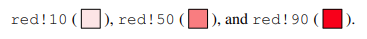
It is important to annotation that the xcolor package — which was mentioned in Subsection 3.2: Colours — offers a more concise though slightly less readable way of making colours transparent. When using a colour, an exclamation mark can be used afterwards the colour name, right after which comes the opacity value — color proper noun!opacity value. This one ranges from 0 being perfectly transparent to 100 being perfectly opaque. For instance, carmine!10 is mostly transparent, reddish!l is half transparent, and reddish!90 is mostly opaque. (Although, if I might add, that "by and large transparent cherry" looks more like salmon.)
5.two. Shading in boxes with colours
Now that nosotros have distinguished which supply bend is the new ane (more than than just using the characterization S′), nosotros also want to indicate the areas that represent the total revenue loss and the total revenue gain for the farmers. That fashion, we can graphically show that the loss in total revenue is much greater than the total revenue proceeds. The command that fills in an expanse on the graph with colour takes the form of:
In this command, (A), (B), (C), . . . , are an indefinite number of coordinates. The command colours in the polygon defined by the coordinates with the specified color. Looking at the graph, the original equilibrium point is (5.five, seven.67) and the new equilibrium betoken is (7, 3.67). Meaning that, for the loss area, we need to colour in orangish the square defined by the coordinates (0, 7.67), (0, iii.67), (five.v, 3.67), and (five.5, 7.67). Similarly, we shade green the gain area defined past the coordinates (5.5, 0), (five.5, iii.67), (seven, 3.67), and (7, 0). So far, we have the post-obit code snippet:
Since we desire these coloured areas to be unobtrusive, the colours demand to exist by and large transparent. This can be done the aforementioned way it is done to plots every bit shown in the previous subsection, Subsection 5.1: Opacity and transparency, either through TikZ'due south opacity parameter or through xcolor's exclamation marker note. So the snippet the graph volition be using is:
Unfortunately, we cannot simply put these commands into the centrality environment. At that place are a couple considerations to address then that these coloured areas do not interfere and overlap with other features on the graph. Because pgfplots processes commands sequentially and then that later plots are layered upon before plots, the fill commands should precede every other one — otherwise the coloured areas could encompass upwardly some other part of the graph. Besides, since fill commands cannot precede the axis parameters, the centrality parameter axis on top should be added. This ensures that the axis lines are non covered up by plots and other commands. The coloured areas are shown in Effigy 5–3.
5.three. Straight and curly arrows
While this graph illustrates the bumper harvest through the relative sizes of the shaded areas, it is missing data almost what those shaded areas represent. Of course, a reader could infer from context that the orange area represents the total revenue loss and the dark-green area represents the total revenue proceeds, just nosotros can also make the graph more readable for them. So let usa label the shaded areas with curly arrows. Also, since nosotros want to illustrate the supply curve moving from the original to the new one, we tin depict a straight arrow from the original to the new curves.
Starting with the latter, since that is easier, the command for drawing arrows takes the course of:
This command draws an arrow starting from (A) and ending at (B). The tip of the pointer at B is specified by the arrowhead value. TikZ has a limited array of arrowheads to cull from, so that is why we loaded the arrows.meta TikZ library in Subsection 1.3: Packages. With this library, we have access to more arrowheads such every bit Triangle, Circumvolve, Square, Diamond, and then on, all of which are self-descriptive. The Triangle arrowhead is the nigh appropriate to show the shift from the original to the new supply curves.
Using this command, we volition draw an arrow from the right of the original supply curve to the left of the new supply bend. This corresponds to an arrow from (6.3, 8.v) to (8.three, 8.v) with an arrowhead of Triangle. Then we have the following code snippet:
While this will do the job, there are a couple changes we should make to amend the aesthetics and readability of the arrow. First, it would exist better if the arrow was a mostly transparent red to show it is modifying the supply bend. Conveniently, this is only like filling areas with colours and colouring plots as we take done in before. Nosotros write scarlet, opacity = 0.3 every bit parameters to the depict command for the arrow. 2nd, arrowheads are small past default. We would similar to brand the supply bend shift arrow slightly bigger. This is slightly harder to exercise. To begin with, we surround the arrowhead value with curly braces to indicate that we are using a custom arrowhead. So we have -{Triangle}. Then, as parameters to the arrowhead value we add the parameters length = 4mm, width = 2mm which modify the dimensions of the arrowhead. Accordingly, we take the last code snippet for the supply shift pointer:
Using this command to draw the pointer upon the graph results in Effigy 5–iv.
Side by side, we will characterization the gain and loss areas. Merely putting a vertical pointer from below the ten-centrality to the green expanse would be too cluttered. We would take the labels Q, Q′ , and an pointer all sharing that small-scale space. Instead, permit united states describe a curly arrow pointing from the bottom-right of the centrality to the eye of the greenish area curving in a counterclockwise direction and then that it avoids the Q and Q′ labels. Curly arrows are drawn with a draw control in the grade of:
Notice that this is nearly identical to the control for straight arrows, except for one add-on. Within the foursquare brackets after the "to", the parameters specify the angles from the starting coordinate and to the ending coordinate which the line for the curve should exist fatigued. They are given in arc degrees, significant from 0 for correct, to 90 for up, to 180 for left, to 270 for downwards, to 360 for correct over again, and everything in between. I have institute beforehand that the starting coordinate for the curly arrow is (10, -1.five) and the ending coordinate is (vi.v, 0.seven). Since the arrow should spring forth up from the starting coordinate and comes into the ending coordinate from the right, the out angle is xc and the in angle is 0. And and so the code snippet producing the curly arrow pointing at the gain area is:
Repeating this for the loss expanse, for an pointer from the height to the orangish box, and adding text labels (which was covered in Subsection iii.five: Labelling), we have this lawmaking snippet:
Combining the directly and curly arrows, Figure 5–5 is produced.
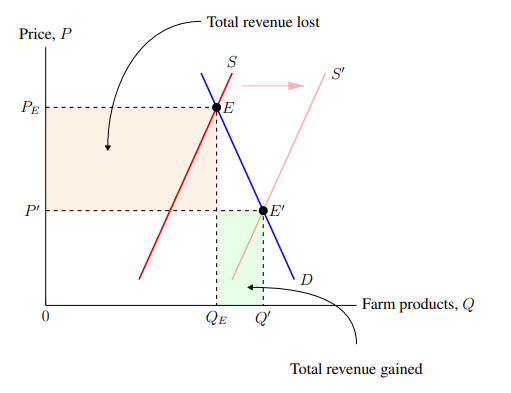
Figure 5–5 is produced past the following code:
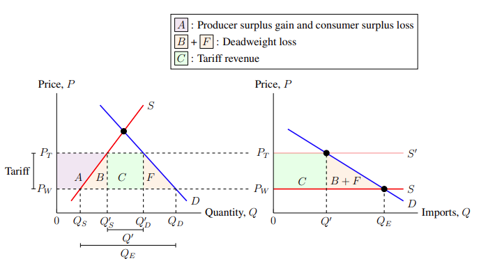
five.four. Arranging graphs side by side
In economic science, information technology is common to adapt the market equilibrium graph to exist next with the price-taking business firm graph. This is useful to show how shifts in the market sets the price with which individual firms need to operate. More generally, we will employ this example to demonstrate how we tin identify graphs beside each other. Suppose we wanted to show how the downward price motion in the market equilibrium causes a decrease in the total economic profit for private farmers. The toll-taking graph of this scenario is shown in Figure 5–vi.
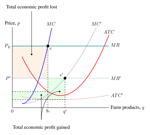
The to a higher place graph is produced entirely with the tools and techniques already covered in previous sections. It is a combination of plots, coordinate points, labels, colours and transparency, and so on. Effigy 5–half dozen is produced by the following lawmaking:
We want it bundled such that the marketplace equilibrium graph (Figure 5–5) is on the left-paw side of a panel while the price-taking firm (Figure 5–6) is on the righthand side. Surprisingly, this is really very simple. All we need to do is create another axis environment right after the first i, only even so within the same tikzpicture environment. This will overlay the two graphs on height of each other. Then, we add the parameter shift = (axis cs: x-shift, y-shift) to the second axis environment where the ten and y-shifts are the amounts by which the second graph will exist moved away from its original position. Since nosotros want to shift the 2d graph (the price-taking firm) to the correct of the showtime graph (the marketplace equilibrium), nosotros will use an x-shift of 17 and a y-shift of 0. And then we accept:
Finally, we need to make an adjustment to fit the figure on the page. Since the figure's width is greater than what the page margins allow, nosotros tell TikZ to disregard the folio margins past widening the picture frame. To do this, we write \hspace*{-3cm} earlier the \brainstorm{tikzpicture} and subsequently the \finish{tikzpicture} which widens the picture's frame to the left by 3 cm and to the correct by 3 cm respectively. In total, putting all of this together yields Effigy v–vii.
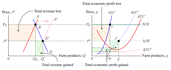
The code that produces Figure 5–7 is:
The lawmaking is executed using the commands and parameters that produce Figures v–five and five–6 for Graphs 1 and ii respectively. (Again, the full code for Figure 5–seven tin be accessed on the GitHub repository https://github.com/jackypacky/pgf-econ-graphs.)
5.5. Shading in the area under a curve
Closing off this section, we will briefly discuss how to shade the area nether a curve — and by extension, how to shade in area betwixt two curves — since that was non covered in the previous example. Suppose we wanted to shade in the surface area nether a production-possibility borderland between good A and skillful B with a transparent blue in order to illustrate the output possibilities that exist which are not necessarily efficient. The production-possibility frontier is illustrated in Figure five–8.
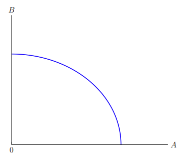
The code that produces Effigy 5–8 is:
To shade in areas betwixt 2 functions, we use a command that takes the form of:
where parameters are the parameters which modify the addplot command, and f and g are the name paths of the functions. For the parameters, nosotros will utilise blueish, and opacity = 0.1 which creates a transparent blue like to what we did in Subsection 5.i: Opacity and transparency.
To input the name paths f and g, yet, we first demand to ascertain the proper name paths beforehand. To define the proper noun path of a curve, we add together the parameter proper noun path = characterization to the addplot command where characterization is the name nosotros desire to assign information technology. And so we will use the addplot parameter proper noun path = frontier for the command which plots the production-possibility curve. Since we need another office betwixt which we can shade in the expanse, and since we want to shade the area under the curve, we demand to plot a new curve divers by the equation y = 0 and proper name it axis. For this new centrality curve, nosotros add together the addplot parameter line width = 0pt to make it invisible — since nosotros exercise not want it to show up on the graph.
In total, shading in the area nether the production-possibility curve is shown in Figure 5–nine.

Effigy 5–ix is produced past the following code:
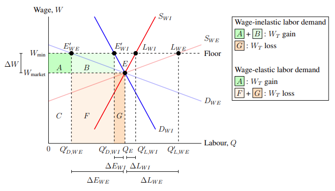
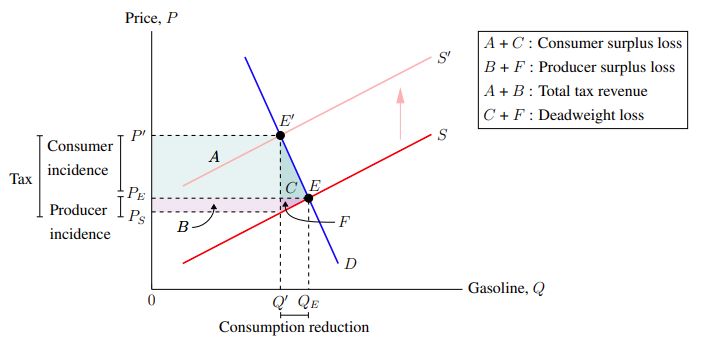
6. Axis dimension lines, line breaks in labels, and a legend (ex. excise tax)
Standing our discussion on enhancing the readability of graphs, let united states of america now impose dimension lines and a legend upon a graph. Instead of putting a characterization on a graph pointing to the coloured areas, we could take instead added a legend showing what each expanse represents. In add-on, to signal what the differences between 2 axis labels are and mean, dimension lines can be used. Dimension lines are lines used in graphs, figures, and drawings to signal sizes, quantities, and distances — dimensions. At each of the ends of dimension lines, there is a perpendicular line joined to it like a "T". (Dimension lines kind of wait like this: "| — –|".)
We will use an excise taxation graph to illustrate the usefulness of dimension lines. Suppose we wanted to illustrate the tax incidence of an excise tax on gasoline. This is shown in Figure 6–i.
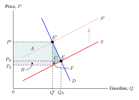
The code that produces Figure half dozen–1 is:
6.1. Calculation dimension lines and line breaks in labels
Dimension lines are added in an identical mode to which arrows are drawn. Call up that the command for an arrow takes the class of:
What I did not tell you was that arrowheads tin be appended to both the terminate of an arrow and the start of an pointer. And so the arrow with an arrowhead at its tail and head takes the form of:
Dimension lines use the arrowhead "|", which is a squeamish symbolic clarification of how the pointer looks. We have:
The departure between Qₑ and Q′ is the reduction of the quantity of gas consumed after the imposition of the excise revenue enhancement. To illustrate that on the graph, we will describe a dimension indicator from the bottom of Q′ to Qₑ. Below this, nosotros volition add a characterization with the text "Consumption reduction." Since Q′ is at Q = 4.14 and Qₑ is at Q = 5.05, nosotros have:
Nosotros would like to repeat this for the consumer incidence — between Pₑ and P′ — and the producer incidence — between Pₛ and Pₑ. However, only copying the in a higher place would not work because the label width would be too big. Instead, we need a manner to insert a line suspension between the two words in both labels. This is done past calculation the parameter align = left to tell how the stacked text should align (either left, right, or centre), and by adding two backslashes — "\\" — where nosotros want the line to pause. Accordingly, the lawmaking for dimension lines and labels for the consumer and producer incidences is:
Adding a dimension line from Pₛ to P′ representing the total revenue enhancement and adding all of the dimension lines and labels mentioned so far results in Figure 6–2.

6.2. Adding a legend
Using a legend, we can specify what the areas A, B, C, and F represent on the graph. Adding a legend combines a couple of the commands and parameters used in the terminal subsection. While pgfplots has its own inbuilt fable feature, information technology is rather unwieldy to use. Instead, we are going to use a text label and put it at the top-right of the graph. The label should let line breaks and have a black border drawn effectually it. And so nosotros will use:
Call back that adding the parameter marshal to the node command allows line break — using \\ — to be used within the label. Also, since the align is gear up to left, text lines will be flushed to the left. These were covered in the previous subsection. What is new, even so, is the draw node parameter, which draws a black border effectually the characterization. In the command, the meridian-left of the legend will exist at (10.5, 10), which corresponds to the pinnacle-right of the graph — where we desire the fable to get. Adding text that describes what the areas represent, we have:
Using the above node command to add a legend to the graph, we become Figure half-dozen–3.
As it stands, the legend looks a bit boring. To amend the aesthetics of the fable, we could add a colored background to the letters A, B, C, and F, to visually connect it to the coloured areas which they point to. It would look good if A were coloured a very transparent teal, B were coloured a very transparent violet, and so on.
Fortunately, the xcolor packet has a command to do exactly that. The xcolor command to add together a coloured background to text takes the grade of:
In this command, the frame colour is the color which surrounds the edges of the coloured background. The groundwork colour is the colour behind the text. For the A text in the fable, since nosotros want its groundwork to be a very transparent teal, the command we want is:
Notice that the command does not stop with a semicolon, this is because information technology is not a TikZ control.

While the A looks fine, the widths of the background colour is determined past the widths of the text within it. So we hitting a snag when using multiple background colours for texts with varying widths. For example, the background color for M is wider than the one for l. Abreast each other, the inconsistent widths are noticeable. To fix this, nosotros will use the makebox LaTeX command (\makebox[width]{text}) with the width of the height of "X", (\fontcharht\font`10). Meaning the command nosotros volition be using to make a coloured background for the letters is:
which is quite overwhelming to wait at without processing it in parts.

You lot may exist unfamiliar with the grave accent, " ` ". On a conventional US keyboard, information technology is located at the peak-left. It is used in LaTeX for an assortment of purposes, including quotation marks and adding a grave accent to characters. (For instance, adding a grave emphasis to "a" using \`a produces "à".)This fashion, 1000 is only as wide as 50. Unfortunately, controlling heights is much harder and I will skip it in this guide. If nosotros wanted to but accept a coloured box with no text in it, we would utilize:
Running the above control produces a transparent teal coloured box.

This works considering \rule{width}{acme} generates a rectangular blob of ink. Incidentally, this is how I have been presenting the colours on their own throughout this guide. Finally, because adding a legend ofttimes makes a graph'due south width bigger than what the page margins allow, we add \hspace*{-3cm} before \begin{tikzpicture} and afterward \end{tikzpicture}. Nosotros too did this in Subsection 5.4: Arranging graphs side by side when we encountered the same problem.
In total, we have the following lawmaking snippet for the fable:
Calculation this to the graph, we become Figure 6–4.
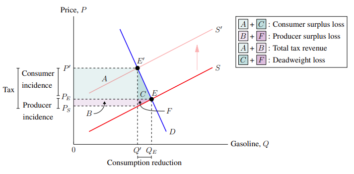
And viola! We have added dimension lines and a fable, further communicating what different sections of the graph mean. Now, anyone looking at this graph would pictorially understand that consumers acquit the bulk of the tax incidence and the surplus loss from a gasoline excise taxation — and why. (Assuming that supply is relatively cost-rubberband and demand is relatively price-inelastic.) The code that produces Figure 6–4 is:
seven. Decision
With this toolbox, you lot tin create almost any economic graph. The try to learn pgfplots and LaTeX is worth it. While on one paw, about word processors such equally Google Docs (with Google Sheets) and Word (with Excel) can provide the necessities of economical graphs — axes, lines, curves, and labels — pgfplots has more flexibility, from shading areas, to calculation dashed lines, and to adding dimension lines. All done in style.
Of grade, since information technology is LaTeX, this is just the tip of the iceburg. Everyone stands on the shoulders of giants. First, Donald Knuth created TeX to typeset documents. Then Leslie Lamport created LaTeX equally a markup to TeX. Then Till Tantau created TikZ on summit of this foundation to create graphics. Afterwards, before, and between this sequence is a list of many other contributors to the giant on which we stand. Finally, we come along and, with serendipity, find out that nosotros tin can create cute and sleek graphs for economics.
Nonetheless, we can ever do more. For case, we could automate the graph cosmos by defining variables and automatically calculating the points of intersection. That, however, is outside the scope of this guide.
If I have washed my job successfully, you accept partially scaled LaTeX's reputable learning curve in this 1 domain of making graphs. If I have not, you have been left abandoned, with no guidance on how to begin your ascent (at least, not from me!). Let us hope for the sometime.
8. Resources
Getting started with LaTeX and learning
- TeX Live: http://world wide web.tug.org/texlive/. This is a portal to install TeX, the TeXworks IDE, and a few ubiquitous packages (including pgfplots and xcolor).
- Overleaf: https://world wide web.overleaf.com/. If installing LaTeX is likewise much of a commitment, there are many online LaTeX editors that are sufficient for this guide. Overleaf has pgfplots and xcolor already installed, so yous do not need to worry about that. On the subject of pricing, they offer a free version which contains all the essentials and only lacks a few specialized features such as GitHub integration or real-time collaboration.
- LaTeX on Wikibooks: https://en.wikibooks.org/wiki/LaTeX. This guide explains the basics of how LaTeX works. From installing LaTeX, to making a document, to more than technical aspects such as boxes, the Wikibook has its explanations and accompanying code.
- TeX-LaTeX Stack Exchange: https://tex.stackexchange.com/. Stack Commutation is a forum where people can ask and answer questions. This subforum specifically deals with LaTeX, which includes pgfplots. Of grade, if you take a question, kickoff use the search characteristic to check if it has been answered before. Then, read the rules and enquire abroad.
Pgfplots and TikZ guides
- Pgfplots packet guide by Overleaf: https://www.overleaf.com/learn/latex/Pgfplots_package. Pgfplots was designed to brand line graphs and scatter plots. We had to adapt it for economic graphs. But if you want to utilise pgfplots for more conventional purposes, read this guide by Overleaf.
- Usepackage{TikZ} for economists by Kevin Goulding: http://static.latexstudio.internet/wp-content/uploads/2016/06/tikzforeconomists-110619150244-phpapp01.pdf. This is another guide on making economic graphs in LaTeX. Information technology uses TikZ, even so, and was written before pgfplots was released. Since pgfplots is a dependency of TikZ, the lawmaking explained in Kevin Goulding's guide may be applicable to making economic graphs with pgfplots.
Package installation links and documentation
Although the LaTeX editing solutions higher up — TeX Live and Overleaf — already have these packages pre-installed, if you do not have these packages or desire the latest versions, you tin can access them at these CTAN links. Too, package manuals are available on CTAN, but beware they are hundreds of pages of technical documentation.
- Pgfplots package on CTAN: https://ctan.org/pkg/pgfplots. This pgfplots bundle installation link also comes with TikZ.
- Xcolor bundle on CTAN: https://ctan.org/pkg/xcolor.
9. Other examples
Again, all of the finished graphs in this guide — the PDFs and the lawmaking — are available on the GitHub repository, including the examples below. The repository can be accessed at https://github.com/jackypacky/pgf-econ-graphs.

Source: https://towardsdatascience.com/using-pgfplots-to-make-economic-graphs-in-latex-bcdc8e27c0eb
Posted by: blumejoad1947.blogspot.com
0 Response to "How To Draw Economic Graphs In Word"
Post a Comment